Axions in CLASSpp: exact scalar-field treatment and the pheno-axion EDE fluid

Summary and test of changes in PR #370 — branch axion-species.

This notebook is a short report on the two axion components added to CLASSpp, following Vivian Poulin’s AxiCLASS as the physics reference (Poulin et al. arXiv:1806.10608, arXiv:1811.04083; Smith et al. arXiv:1905.12618):

1. An exact axion potential for ScalarFieldSpecies — the Klein–Gordon equation is integrated throughout, valid whenever the field oscillates slowly enough for the ODE to resolve (axion dark energy, late oscillation onset).

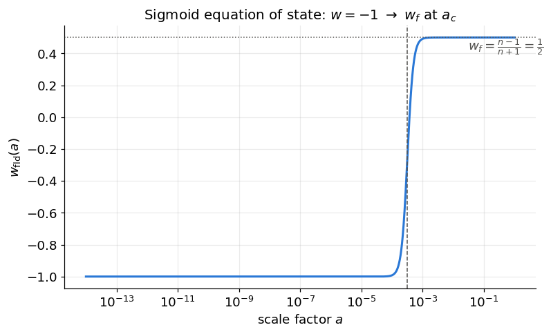
2. The pheno-axion effective early-dark-energy (EDE) fluid — AxiCLASS’s pheno_axion parametrization: a fluid whose equation of state transitions from \(w_i=-1\) to \(w_f=\frac{n-1}{n+1}\) at scale factor \(a_c\), with the Poulin et al. scale-dependent effective sound speed. This is the numerically cheap parametrization used in published EDE analyses, valid deep in the oscillatory regime where the exact treatment is intractable.

Design spec: docs/superpowers/specs/2026-07-14-axion-species-design.md. Both features are strictly opt-in: default CLASSpp output is unchanged.

1. Physics background

An axion-like field \(\phi\) with decay constant \(f\) has the potential

\[V(\phi) = m^2 f^2 \left(1-\cos\frac{\phi}{f}\right)^n ,\]

which is \(\tfrac12 m^2\phi^2\)-like near the minimum for \(n=1\) and flattens for larger \(n\). Hubble friction freezes the field at its initial misalignment angle \(\Theta_i = \phi_i/f\) until \(H(a)\) drops to \(\mathcal{O}(m)\); it then rolls and oscillates. Averaged over oscillations the energy density dilutes as \(\rho\propto a^{-3(1+w_n)}\) with \(w_n = \frac{n-1}{n+1}\) (Turner 1983): \(n=1\) behaves like matter, \(n=2\) like radiation, \(n=3\) dilutes faster than radiation (\(w=1/2\)) — the property that makes \(n\geq 2\) axions interesting as early dark energy resolving the \(H_0\) tension.

Two regimes, two tools. From oscillation onset to today the field completes \(\sim m/H_0\) cycles; for the canonical EDE transition (\(a_c\sim10^{-3.5}\)) that is \(10^5\)–\(10^6\) oscillations per Fourier mode — hopeless for a direct ODE integration. Component 1 therefore covers the slow regime exactly, and component 2 covers the deep-oscillation regime with the effective fluid.

For the fluid, the background equation of state is the sigmoid (“mash-up of 1811.04083 and 1905.12618”)

\[w(a) = w_i + \frac{w_f-w_i}{1+(a_c/a)^{r}},\qquad r = \frac{3(w_f-w_i)}{\nu},\]

whose density integral \(\int_a^1 3\,\frac{1+w}{a'}\,\mathrm{d}a'\) has a closed form — all density normalizations (\(\Omega_{\rm fld,0}\leftrightarrow\Omega_{\rm fld}(a_c) \leftrightarrow f_{\rm EDE}(a_c)\)) are algebraic, no shooting involved. Perturbations use the true fluid equations with the generalized-dark-matter effective sound speed (1806.10608, Eq. 20)

\[c_s^2(k,a) = \frac{2a^2(n-1)\,\varpi^2 + k^2}{2a^2(n+1)\,\varpi^2 + k^2}, \qquad \varpi(a) \equiv \omega_{\rm axion}\, a^{-3(n-1)/(n+1)},\]

where \(\omega_{\rm axion}\) is calibrated from \((a_c,\,\Omega_{\rm fld}(a_c),\,\Theta_i,\,n)\) per Eqs. 27/28/30 of 1806.10608.

import numpy as np
import matplotlib
import matplotlib.pyplot as plt
from classy import Class

# House style: recessive grid/axes, thin marks, validated categorical palette
# (slots in fixed order; see PR #370 notes).
C1, C2, C3, C6 = "#2a78d6", "#1baf7a", "#eda100", "#e34948"
NEUTRAL = "#52514e"
matplotlib.rcParams.update({
    "figure.figsize": (8.0, 4.5), "figure.dpi": 110,
    "lines.linewidth": 2.0, "axes.grid": True, "grid.alpha": 0.25,
    "axes.spines.top": False, "axes.spines.right": False,
    "font.size": 12, "axes.titlesize": 13, "legend.frameon": False,
})

BASE = {"h": 0.67, "omega_b": 0.02238, "omega_cdm": 0.1201}

def run(extra, level=None, lmax=2500):
    cosmo = Class()
    cosmo.set({**BASE, **extra})
    cosmo.compute() if level is None else cosmo.compute(level=level)
    return cosmo

2. Component 1 — exact axion scalar field

Input keys (explanatory.ini documents all of them):

key	meaning
scf_potential = axion	selects the \((1-\cos)^n\) potential bundle
f_axion	decay constant \(f\) (reduced-Planck units, required)
n_axion	exponent \(n\ge1\) (default 1)
Theta_initial_scf	misalignment angle \(\Theta_i\in(0,\pi)\); frozen ICs \(\phi_i=\Theta_i f\), \(\phi_i'=0\)
m_axion	optional Newton seed (1/Mpc)
Omega_scf	shooting target — \(m\) is always tuned so that \(\Omega_{\rm scf}\) today matches

The second derivative of the potential is implemented in the regular form \(V'' = m^2 n\, u^{n-1}\left[(n-1)(2-u) + (1-u)\right]\) with \(u=1-\cos(\phi/f)\) (using \(\sin^2 = u(2-u)\)), which is finite at the minimum for all \(n\ge1\) — the AxiCLASS expression is singular there for \(n=1\) and was deliberately not ported.

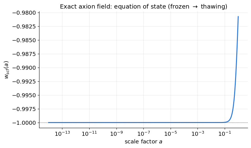
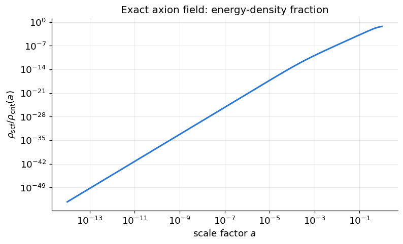
Below: an axion-dark-energy configuration (\(n=1\), \(f=0.5\,M_{\rm P}\), \(\Theta_i=2\), \(\Omega_{\rm scf}=0.05\)). The shooting resolves \(m\simeq0.7H_0\): the field is frozen (\(w\simeq-1\)) through recombination and only begins to thaw today.

scf = run({"scf_potential": "axion", "f_axion": 0.5, "n_axion": 1,
           "Theta_initial_scf": 2.0, "Omega_scf": 0.05}, level=["background"])
bg = scf.get_background()
a = 1.0 / (1.0 + bg["z"])
o = np.argsort(a)
a_s = a[o]
w_scf = (bg["(.)p_scf"] / bg["(.)rho_scf"])[o]
f_scf = (bg["(.)rho_scf"] / bg["H [1/Mpc]"] ** 2)[o]

omega_today = f_scf[-1]
print(f"shooting hit: Omega_scf(a=1) = {omega_today:.7f}  (target 0.05)")

shooting hit: Omega_scf(a=1) = 0.0500003  (target 0.05)

fig, ax = plt.subplots()
ax.semilogx(a_s, w_scf, color=C1)
ax.set(xlabel=r"scale factor $a$", ylabel=r"$w_{\rm scf}(a)$",
       title=r"Exact axion field: equation of state (frozen $\to$ thawing)")
ax.axhline(-1, color=NEUTRAL, lw=1, ls=":")
ax.annotate(r"frozen, $w=-1$", xy=(1e-4, -0.97), color=NEUTRAL)
plt.show()

fig, ax = plt.subplots()
ax.loglog(a_s, f_scf, color=C1)
ax.set(xlabel=r"scale factor $a$", ylabel=r"$\rho_{\rm scf}/\rho_{\rm crit}(a)$",
       title="Exact axion field: energy-density fraction")
plt.show()
scf.struct_cleanup(); scf.empty()

<classy.Class at 0x7808bbc4bbc0>

3. Component 2 — pheno-axion EDE fluid: background

Input keys: fluid_equation_of_state = pheno_axion; n_pheno_axion xor w_fld_f; a_c xor log10_axion_ac; exactly one of Omega_fld / Omega_fld_ac / fraction_fld_ac; Theta_initial_fld (required); nu_fld (default 1); w_fld_i (default \(-1\)). The keys match AxiCLASS so existing .ini files port directly. use_ppf and cs2_fld are rejected — PPF is meaningless here (\(w>-1\) for all \(a>0\)) and the sound speed is derived, not an input.

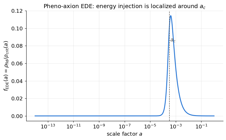
We use the canonical EDE benchmark throughout: \(n=3\), \(\log_{10}a_c=-3.5\), \(f_{\rm EDE}(a_c)=0.1\), \(\Theta_i=2.8\).

EDE = {"fluid_equation_of_state": "pheno_axion", "n_pheno_axion": 3,
       "log10_axion_ac": -3.5, "fraction_fld_ac": 0.1, "Theta_initial_fld": 2.8}
a_c = 10 ** -3.5

ede_bg = run(EDE, level=["background"])
bg = ede_bg.get_background()
a = 1.0 / (1.0 + bg["z"]); o = np.argsort(a); a_s = a[o]
f_ede = (bg["(.)rho_fld"] / bg["H [1/Mpc]"] ** 2)[o]
w_fld = bg["(.)w_fld"][o]

f_at_ac = np.interp(a_c, a_s, f_ede)
i_pk = np.argmax(f_ede)
print(f"f_EDE(a_c) = {f_at_ac:.7f}   (input fraction_fld_ac = 0.1)")
print(f"peak fraction {f_ede[i_pk]:.4f} at a = {a_s[i_pk]:.2e}  (a_c = {a_c:.2e})")

f_EDE(a_c) = 0.1000004   (input fraction_fld_ac = 0.1)
peak fraction 0.1143 at a = 4.10e-04  (a_c = 3.16e-04)

fig, ax = plt.subplots()
ax.semilogx(a_s, f_ede, color=C1)
ax.axvline(a_c, color=NEUTRAL, lw=1, ls="--")
ax.annotate(r"$a_c$", xy=(a_c * 1.15, 0.085), color=NEUTRAL)
ax.set(xlabel=r"scale factor $a$", ylabel=r"$f_{\rm EDE}(a)=\rho_{\rm fld}/\rho_{\rm crit}(a)$",
       title="Pheno-axion EDE: energy injection is localized around $a_c$")
plt.show()

fig, ax = plt.subplots()
ax.semilogx(a_s, w_fld, color=C1)
ax.axvline(a_c, color=NEUTRAL, lw=1, ls="--")
ax.axhline(0.5, color=NEUTRAL, lw=1, ls=":")
ax.annotate(r"$w_f=\frac{n-1}{n+1}=\frac{1}{2}$", xy=(3e-2, 0.42), color=NEUTRAL)
ax.set(xlabel=r"scale factor $a$", ylabel=r"$w_{\rm fld}(a)$",
       title=r"Sigmoid equation of state: $w=-1\ \to\ w_f$ at $a_c$")
plt.show()
ede_bg.struct_cleanup(); ede_bg.empty()

<classy.Class at 0x7808bb30c120>

The background behavior matches theory to high precision (numbers from the PR’s validation suite, reproduced by the cell above): the plateau is flat to \(2\times10^{-7}\), the dilution tail scales as \(a^{-4.500}\) (\(-3(1+w_f)=-4.5\) exactly), and \(f_{\rm EDE}(a_c)\) reproduces the input fraction to \(4\times10^{-7}\) — the \(\Omega_{\rm fld,0}\leftrightarrow f_{\rm EDE}(a_c)\) conversion is exact for the fluid itself (closed-form integral), with only the neutrino-scaling approximation of \(\Omega_{\rm tot}(a_c)\) entering the fraction definition.

4. Impact on the CMB

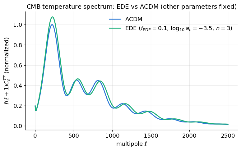
The canonical EDE point shifts the acoustic peaks — the classic EDE signature (extra energy density around matter–radiation equality shrinks the sound horizon; with all other parameters held fixed the peaks move).

lcdm = run({"output": "tCl"})
ede = run({**EDE, "output": "tCl"})

cl0 = lcdm.raw_cl(2500)
cl1 = ede.raw_cl(2500)
ell = cl0["ell"][2:]
dl0 = cl0["tt"][2:] * ell * (ell + 1)
dl1 = cl1["tt"][2:] * ell * (ell + 1)

fig, ax = plt.subplots()
ax.plot(ell, dl0 / dl0.max(), color=C1, label=r"$\Lambda$CDM")
ax.plot(ell, dl1 / dl0.max(), color=C2, label=r"EDE ($f_{\rm EDE}=0.1$, $\log_{10}a_c=-3.5$, $n=3$)")
ax.set(xlabel=r"multipole $\ell$", ylabel=r"$\ell(\ell+1)C_\ell^{TT}$ (normalized)",
       title="CMB temperature spectrum: EDE vs $\\Lambda$CDM (other parameters fixed)")
ax.legend()
plt.show()

fig, ax = plt.subplots()
ax.plot(ell, 100 * (dl1 / dl0 - 1), color=C1)
ax.axhline(0, color=NEUTRAL, lw=1, ls=":")
ax.set(xlabel=r"multipole $\ell$", ylabel=r"$\Delta C_\ell^{TT}/C_\ell^{TT}$  [%]",
       title="Fractional change: median $\\sim$9%, up to $\\sim$40% at the peak shifts")
plt.show()
med = np.median(np.abs(dl1 / dl0 - 1)); mx = np.max(np.abs(dl1 / dl0 - 1))
print(f"median |dCl/Cl| = {med:.3f},  max = {mx:.3f} at l = {ell[np.argmax(np.abs(dl1/dl0-1))]}")

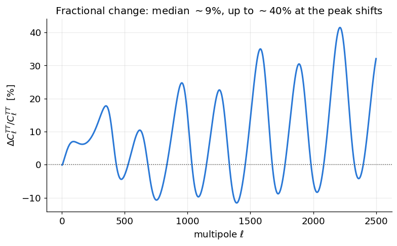
median |dCl/Cl| = 0.087,  max = 0.415 at l = 2213

5. Consistency checks

Decoupling. Sending the EDE fraction to \(10^{-8}\) must reproduce \(\Lambda\)CDM. The residual is at the \(2\times10^{-5}\) level — numerical noise, far below cosmic variance.

tiny = run({**EDE, "fraction_fld_ac": 1e-8, "output": "tCl"})
clt = tiny.raw_cl(2500)
ratio = np.abs(clt["tt"][2:] / cl0["tt"][2:] - 1)

fig, ax = plt.subplots()
ax.semilogy(ell, ratio, color=C1)
ax.axhline(1e-4, color=NEUTRAL, lw=1, ls="--")
ax.annotate("acceptance threshold $10^{-4}$", xy=(60, 1.4e-4), color=NEUTRAL)
ax.set(xlabel=r"multipole $\ell$", ylabel=r"$|C_\ell^{\rm tiny}/C_\ell^{\Lambda\rm CDM}-1|$",
       title=r"Decoupling: $f_{\rm EDE}\to10^{-8}$ recovers $\Lambda$CDM")
plt.show()
print(f"max residual = {ratio.max():.2e}")
for c in (lcdm, ede, tiny):
    c.struct_cleanup(); c.empty()

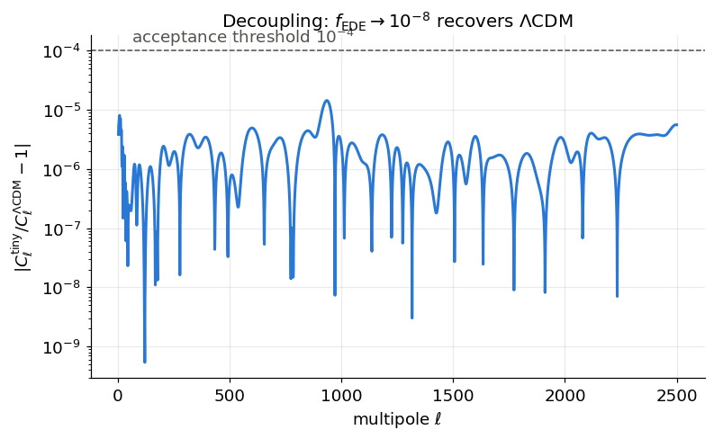
max residual = 1.44e-05

Guard rails. Integration testing surfaced two pre-existing module checks that were incompatible with a fluid whose \(w\to-1\) asymptotically; both are now species-owned virtuals (see PR #370):

• FluidSpecies::ReachesPhantomDivide() — the historical perturb_init test fired on the exact \(w(a{=}0)=-1\) asymptote; the sigmoid never reaches \(-1\) at any \(a>0\).

• FluidSpecies::HyrecCplApproximation() — HyRec reconstructs its internal dark-energy density from a single CPL \((w_0,w_a)\) pair (hyrec/history.c), which cannot represent \(\Lambda\) + a frozen\(\to\)diluting sigmoid; pheno-axion runs therefore require recombination = RECFAST (the default, which reads the true background table). HyRec fails fast with an actionable message (proper fix — feeding HyRec the true \(H(z)\) — is issue #369):

from classy import CosmoComputationError
bad = Class()
bad.set({**BASE, **EDE, "output": "tCl", "recombination": "HyRec"})
try:
    bad.compute()
except CosmoComputationError as err:
    msg = str(err)
    print(msg[msg.find("condition"):][:400])
bad.struct_cleanup(); bad.empty()

condition (!fld.HyrecCplApproximation(&param.w0, &param.wa)) is true; this fluid's dark-energy density history cannot be represented by the CPL (w0, wa) pair that HyRec uses internally (hyrec/history.c) — HyRec would misreconstruct H(z) at recombination. Use 'recombination = RECFAST', which reads the true background table.

<classy.Class at 0x7808b92790e0>

6. Validity, limitations and follow-ups

regime	tool	status
frozen / slowly thawing field (\(m \lesssim 10^2 H_0\))	component 1 (exact KG)	✔ this PR
deep-oscillation EDE (\(a_c \ll 1\), \(10^{5+}\) cycles)	component 2 (effective fluid)	✔ this PR
KG \(\to\) fluid runtime switching (AxiCLASS scf_evolve_as_fluid)	—	issue #365
axion inside the Type-3 momentum-transfer composite	—	issue #366
\(f_{\rm EDE}\)-peak derived parameters via the wrapper	—	issue #367
phi_2n / axionquad potentials	—	issue #368
HyRec with the true \(H(z)\) (also fixes silent scf-DE approximation)	—	issue #369

Two AxiCLASS bugs were deliberately not ported: the C comma-operator slip in the analytic \(\mathrm{d}w/\mathrm{d}a\) (rederived and verified against finite differences) and the \(n=1\)-singular \(V''\) (replaced by the regular form of §2). The unit tests (test-scf-potential, test-axion-scf-factory, test-axion-ede-fluid) verify the potential derivatives against finite differences, the closed-form density integral against quadrature, the \(c_s^2\) limits (\(k\to0\): \(w_f\); \(k\to\infty\): 1), the \(\Omega\) round-trips, and every input-validation rejection branch.

import subprocess
from importlib.metadata import version
print("HEAD:", subprocess.run(["git", "log", "--oneline", "-1"], capture_output=True,
                              text=True, cwd="..").stdout.strip())
print("classy-community", version("classy-community"))

HEAD: 9d91594 dcdm_wdm: injection-adapted quantile momentum grid + conservative erf energy deposit (#384)
classy-community 26.0.0