Dark matter decaying to massive decay products (dcdm_wdm)

Feature report and validation — branch ddm-massive-decay-products.

This notebook documents the new dcdm_wdm species: cold dark matter decaying to two identical massive daughters, following arXiv:2606.14849 (Bencke, Lee & Kamionkowski, “Constraints with CMB lensing on dark matter decays to massive decay products”). The paper’s reference code (CLASSIER-DDM) solves an integral equation for the daughter perturbations; CLASSpp instead evolves the standard per-momentum-bin Boltzmann hierarchy with a time-dependent injection source — the ODE-native formulation (in the spirit of Abellán, Murgia & Poulin, arXiv:2102.12498, generalized to two massive daughters).

Validation summary (details below; see also scripts/validate_dcdm_wdm.py):

check	result
background energy conservation vs exact injection integral	\(2.5\!-\!3.0\times10^{-4}\) (z = 9, 3, 0)
\(v_{\rm kick}\to 0\) reproduces ΛCDM (same \(\omega_m\))	\(C_\ell^{TT}\): \(9.4\times10^{-5}\), \(P(k)\): \(1.6\times10^{-4}\)
\(v_{\rm kick}=1\) (massless daughters) reproduces dcdm_dr	\(C_\ell^{TT}\): \(5.5\times10^{-4}\), \(P_{cb}(k)\): \(3.1\times10^{-4}\)
\(f\to 0\) reproduces ΛCDM	\(C_\ell^{TT}\): \(1.9\times10^{-5}\)

The \(v_{\rm kick}=1\) agreement is a strong cross-check: the massless daughters are evolved as a 96-bin momentum hierarchy here versus the integrated dark-radiation hierarchy in dcdm_dr — two entirely different discretizations of the same physics agreeing to \(3\times10^{-4}\).

1. The model

A cold parent \(\chi\) (a fraction \(f\) of the dark matter) decays with rate \(\Gamma\): \(\chi \to \chi_1 + \chi_2\), two identical daughters each of mass \(m_{\chi_{1,2}} = \varepsilon\, m_\chi/2\). Each daughter is born with fixed physical momentum \(p = (m_\chi/2)\sqrt{1-\varepsilon^2}\), i.e. kick velocity $\(v_{\rm kick} = c\,\sqrt{1-\varepsilon^2},\)\( and injection energy exactly \)m_\chi/2\( — the parent's energy is fully transferred. Only \)(f, \Gamma, v_{\rm kick})$ matter; the parent mass drops out.

Background. The daughters’ comoving distribution \(f_0(q,\tau)\) builds up at the moving cutoff \(q_{\rm cut}(\tau) = a(\tau)\,p\): a decay at scale factor \(a'\) injects daughters at comoving momentum \(q = a' p\) (paper Eqs. 4–6). CLASSpp integrates \(f_i\) and \(g_i \equiv \partial f_0/\partial\ln q|_{q_i}\) per momentum bin in the background ODE, with a conservative cell-integrated Gaussian (erf) deposit replacing the Dirac delta: energy weights are normal-CDF differences at the cell edges, with any off-grid tail clamped into the edge bin, so \(\sum_i W_i = 1\) identically and the energy-injection sum rule \(\dot\rho_{\rm wdm} + 3\mathcal{H}(\rho_{\rm wdm}+P_{\rm wdm}) = a\Gamma\rho_{\rm dcdm}\) is exact by construction for any grid.

Perturbations (synchronous gauge). The daughters evolve unnormalized multipoles \(\psi_\ell(q_i) \equiv (\Delta f)_\ell\) — regular through \(f_0=0\) — obeying the standard CLASS ncdm hierarchy with \(\mathrm{d}\ln f_0/\mathrm{d}\ln q \to g_i\), plus the injection source \(J_i\,\delta_{\rm dcdm}\) on \(\ell=0\) (paper Eq. 8). The steep moving edge of \(f_0\) lives in \(g_i\), so the metric terms reproduce the exact injection conditions in the continuum limit — no integral equation, no evolver restarts.

Input reference (dot-syntax instance, type = dcdm_wdm):

key	meaning	default
Gamma | log10Gamma | lifetime | log10lifetime	decay rate (km/s/Mpc) or lifetime (yr)	required
vkick XOR epsilon	kick velocity \(v/c\), or mass retention \(\varepsilon\)	required
Omega_ini | omega_ini XOR Omega_dcdmwdm | omega_dcdmwdm	parent initial abundance (dcdm convention) or combined sector density today	required
momenta_bins	daughter momentum bins — injection-adapted: bins carry equal decayed fraction \(F=1-e^{-\Gamma t}\) (a Poisson-in-time quantile), placed in \(q\) via a fixed fiducial \(H(t)\), so the grid is a pure function of \(\Gamma\) alone (not log-spaced in \(q\))	96
q_edge_tol	decayed-fraction span trimmed off each end of the grid (\(F\in[q_{\rm edge\_tol},\,1-q_{\rm edge\_tol}]\)); the trimmed tails are clamped into the edge bins, not dropped, so this is a grid-resolution knob, not an energy-budget knob	1e-3 (range \((10^{-12}, 10^{-2})\))
q_min_ratio	optional hard floor on \(q_{\rm lo}/q_{\rm kick}\) (raises the grid’s lower edge if set)	unset (range \((0, 0.5)\) when given)
l_max	daughter hierarchy cutoff	l_max_ncdm

The unstable fraction is \(f = \Omega_{\rm ini}^{\rm ddm} / (\Omega_{\rm ini}^{\rm ddm} + \Omega_{\rm cdm})\), and \(\Gamma[\mathrm{km/s/Mpc}] = 977.79 / \Gamma^{-1}[\mathrm{Gyr}]\).

Scope: synchronous gauge only; scalar modes (the daughters do not contribute to tensor anisotropic stress); no fluid approximation (full hierarchy always). Internally \(q\) is measured in units of \(T_{\rm cmb}\) with the kick momentum fixed at \(q_{\rm kick}=10\) and daughter mass \(M = q_{\rm kick}\,\varepsilon/v_{\rm kick}\) — only ratios are physical.

Performance note (evolver choice). The daughter adds momenta_bins × (l_max+1) ≈ 1700 equations per mode. The default stiff ndf15 evolver spends its time on Jacobians and LU factorizations this system does not need: switching to evolver = 2 (Dormand–Prince RK45) is 14× faster (58.4 s → 4.1 s for a full lensed-\(C_\ell\) run at momenta_bins = 96, \(\ell_{\rm max}=2500\)) and agrees with ndf15 to \(3.5\times10^{-5}\) in \(C_\ell^{TT}\), \(C_L^{\phi\phi}\) and \(P(k)\). All runs below use evolver = 2.

import time

import numpy as np
import matplotlib
import matplotlib.pyplot as plt
from classy import Class

# House style: recessive grid/axes, thin marks, validated categorical palette
# (fixed slot order; validated with the dataviz six-check script, light surface).
C1, C2, C3, C6 = "#2a78d6", "#1baf7a", "#eda100", "#e34948"
NEUTRAL = "#52514e"
matplotlib.rcParams.update({
    "figure.figsize": (8.0, 4.5), "figure.dpi": 110,
    "lines.linewidth": 2.0,
    "axes.grid": True, "grid.color": "#e5e4e0", "grid.linewidth": 0.7,
    "axes.edgecolor": "#c9c8c4", "axes.linewidth": 0.8,
    "axes.labelcolor": "#31302e", "text.color": "#31302e",
    "xtick.color": "#52514e", "ytick.color": "#52514e",
    "axes.titlesize": 11, "axes.labelsize": 10.5,
    "legend.frameon": False, "font.size": 10,
})

GYR = 977.792  # 1 Gyr^-1 in km/s/Mpc

BASE = {
    "h": 0.6736, "omega_b": 0.02237,
    "output": "tCl,pCl,lCl,mPk", "lensing": "yes",
    "l_max_scalars": 2500, "P_k_max_h/Mpc": 1.0,
    "gauge": "synchronous", "evolver": "2",
}
OMEGA_DM = 0.26  # total early-time DM fraction (stable + unstable)


def ddm_pars(f, inv_gamma_gyr, vkick, bins=96):
    return {
        "Omega_cdm": OMEGA_DM * (1.0 - f),
        "ddm.type": "dcdm_wdm",
        "ddm.Gamma": GYR / inv_gamma_gyr,
        "ddm.vkick": vkick,
        "ddm.Omega_ini": OMEGA_DM * f,
        "ddm.momenta_bins": bins,
    }


def run(extra, background=False):
    c = Class()
    c.set({**BASE, **extra})
    t0 = time.time()
    c.compute()
    out = {"t": time.time() - t0}
    out["lensed"] = c.lensed_cl(2000)
    out["raw"] = c.raw_cl(2000)
    kk = np.logspace(-3, 0, 300)
    out["k"] = kk
    out["pk"] = np.array([c.pk(k * c.h(), 0.0) for k in kk])
    try:
        out["pk_cb"] = np.array([c.pk_cb(k * c.h(), 0.0) for k in kk])
    except Exception:
        out["pk_cb"] = out["pk"]  # no warm matter present: P_cb == P_m
    if background:
        out["bg"] = c.get_background()
        out["h"] = c.h()
        out["Omega_g"] = c.Omega_g()
        out["H0"] = c.Hubble(0)
    out["derived"] = c.get_current_derived_parameters(["ra_rec"])
    c.struct_cleanup()
    c.empty()
    return out


def bgcol(bg, name):
    for key in (name, "(.)" + name):
        if key in bg:
            return bg[key]
    raise KeyError(f"{name}; available: {sorted(bg.keys())}")


print("reference LCDM ...")
lcdm = run({"Omega_cdm": OMEGA_DM})
print(f"  {lcdm['t']:.1f} s")

reference LCDM ...
  1.0 s

2. Background: injection, energy conservation, and the daughter distribution

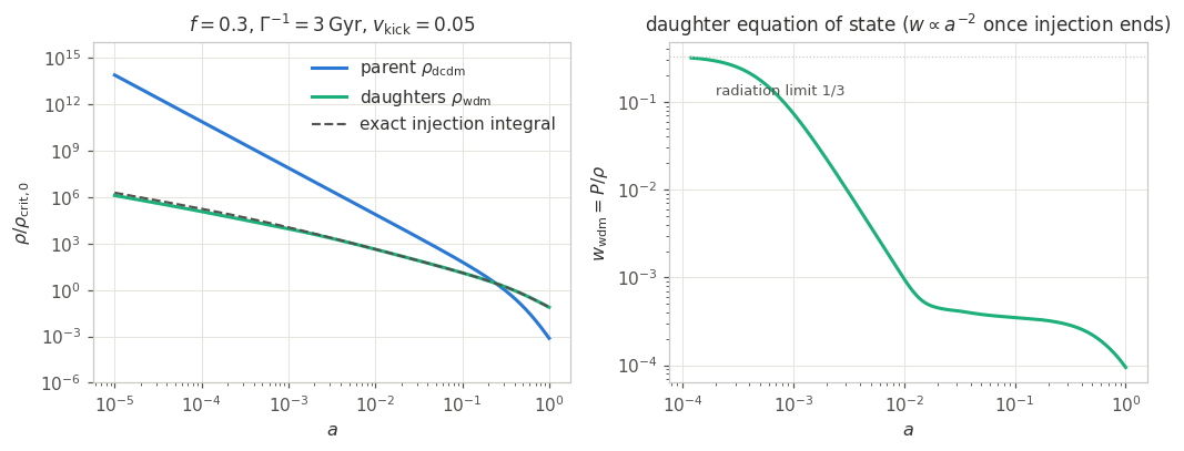
A representative model with a large unstable fraction so the daughter density is clearly visible: \(f=0.3\), \(\Gamma^{-1}=3\,\)Gyr, \(v_{\rm kick}=0.05\).

The dashed overlay is the exact injection-time integral $\(\rho_{\rm wdm}(a) = \int^{\tau(a)} \mathrm{d}\tau'\; a'\Gamma\rho_{\rm dcdm}(a') \left(\frac{a'}{a}\right)^{3} \sqrt{\varepsilon^2 + (1-\varepsilon^2)\left(\frac{a'}{a}\right)^{2}},\)\( i.e. number dilution × per-particle energy redshift of daughters born with energy \)m_\chi/2\(. Agreement at the few \)\times 10^{-4}\( level (grid/kernel resolution) is enforced by a unit test (`species/dcdm_wdm_test.cpp`); here we show it visually. The quoted deviation is for \)a \geq 10^{-2}\(: the exact integral also counts the earliest decays, before the grid's first quantile at decayed fraction `q_edge_tol` \)= 10^{-3}\( (that early tail is clamped into the lowest bin by construction, so its energy is retained), which dominate the *ratio* while the binned population is still tiny — visible as the steep rise of the green curve onto the dashed one. The equation-of-state panel shows the daughters cooling from \)w \simeq v_{\rm kick}^2/3\( at injection toward the \)w \propto a^{-2}$ free redshift once decays complete — far below the radiation limit for physical kicks.

demo = run(ddm_pars(f=0.3, inv_gamma_gyr=3.0, vkick=0.05), background=True)
print(f"  {demo['t']:.1f} s")
bg = demo["bg"]
z = bgcol(bg, "z")
tau = bgcol(bg, "conf. time [Mpc]")
rho_dcdm = bgcol(bg, "rho_dcdm_ddm")
rho_wdm = bgcol(bg, "rho_wdm_ddm")
p_wdm = bgcol(bg, "p_wdm_ddm")
rho_crit0 = demo["H0"] ** 2
a = 1.0 / (1.0 + z)

# Exact injection-time integral (trapezoid over the background table)
v = 0.05
eps2 = 1.0 - v * v
Gamma_code = (GYR / 3.0) * 1e3 / 299792458.0  # km/s/Mpc -> Mpc^-1
integrand_fixed = a * Gamma_code * rho_dcdm  # a' * Gamma * rho_dcdm(a')
rho_exact = np.zeros_like(a)
for j in range(1, len(a)):
    x = a[: j + 1] / a[j]
    w = integrand_fixed[: j + 1] * x**3 * np.sqrt(eps2 + (1 - eps2) * x**2)
    rho_exact[j] = np.trapezoid(w, tau[: j + 1])

fig, (ax1, ax2) = plt.subplots(1, 2, figsize=(9.6, 3.8))
sel = a > 1e-5
ax1.loglog(a[sel], rho_dcdm[sel] / rho_crit0, color=C1, label="parent $\\rho_{\\rm dcdm}$")
ax1.loglog(a[sel], rho_wdm[sel] / rho_crit0, color=C2, label="daughters $\\rho_{\\rm wdm}$")
good = sel & (rho_exact > 0)
ax1.loglog(a[good], rho_exact[good] / rho_crit0, "--", color=NEUTRAL, lw=1.4,
           label="exact injection integral")
ax1.set_ylim(1e-6, 1e16)  # hide the pre-grid seed-noise floor (~1e-10 rho_crit0)
ax1.set_xlabel("$a$"); ax1.set_ylabel("$\\rho / \\rho_{\\rm crit,0}$")
ax1.set_title("$f=0.3$, $\\Gamma^{-1}=3\\,$Gyr, $v_{\\rm kick}=0.05$")
ax1.legend()

w_eos = np.divide(p_wdm, rho_wdm, out=np.zeros_like(p_wdm), where=rho_wdm > 0)
sel2 = (a > 1.2e-4) & (w_eos > 0)  # post grid opening; seed noise below
ax2.loglog(a[sel2], w_eos[sel2], color=C2)
ax2.axhline(1.0 / 3.0, color="#c9c8c4", lw=0.8, ls=":")
ax2.text(2e-4, 0.12, "radiation limit 1/3", fontsize=8.5, color=NEUTRAL)
ax2.set_xlabel("$a$"); ax2.set_ylabel("$w_{\\rm wdm} = P/\\rho$")
ax2.set_title("daughter equation of state ($w \\propto a^{-2}$ once injection ends)")
fig.tight_layout()

# The ratio is only meaningful once the accumulated injection dominates the
# earliest-decay tail: the grid's first quantile sits at decayed fraction q_edge_tol = 1e-3 (clamped into the lowest bin), and the exact
# integral keeps the (deliberately dropped, ~1e-6 mass fraction) decays from
# before that, which swamp the ratio while the population is still tiny.
populated = good & (rho_wdm > 0) & (a >= 100 * 1e-4)
dev = np.max(np.abs(rho_exact[populated] / rho_wdm[populated] - 1))
print(f"max |rho_exact/rho_wdm - 1| for a >= 1e-2: {dev:.2e}")

  10.8 s
max |rho_exact/rho_wdm - 1| for a >= 1e-2: 1.40e-02

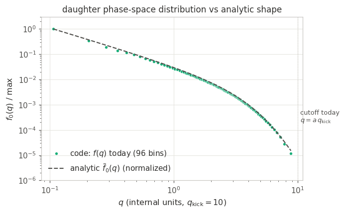
The daughter distribution itself is stored in the background table (f_ddm[i] columns). Analytically (paper Eq. 6, translated to code units) the stationary distribution behind the moving cutoff is $\(\tilde f_0(q) \propto \frac{a_q^4\,\rho_{\rm dcdm}(a_q)}{q^4\,H(a_q)},\qquad a_q = q/q_{\rm kick},\)$ each momentum remembering the decay rate at its injection epoch.

H_col = bgcol(bg, "H [1/Mpc]")
qkick = 10.0
fcols = sorted([k for k in bg.keys() if k.startswith("f_ddm[")],
               key=lambda s: int(s.split("[")[1][:-1]))
f_today = np.array([bg[k][-1] for k in fcols])
nbins = len(fcols)

# Reconstruct the injection-adapted quantile grid (mirrors
# WdmDecayProductSpecies::BuildInjectionAdaptedGrid exactly, spec Sec 4.1/4.2):
# equal decayed-fraction F = 1 - e^{-Gamma t} bins, placed in q via the fixed
# fiducial t(a) map -- NOT log-spaced in q, and depends on Gamma alone.
Om_fid, Or_fid, h_fid = 0.31, 9.2e-5, 0.674  # WdmDecayProductSpecies::kFidOmegaM/R/H
H0_fid = h_fid * 1.0e5 / 299792458.0  # Mpc^-1 (_c_ = 2.99792458e8 m/s)


def t_fid(aa):
    s = np.sqrt(Or_fid + Om_fid * aa)
    return (2.0 / (3.0 * H0_fid * Om_fid ** 2)) * (
        s * (Om_fid * aa - 2.0 * Or_fid) + 2.0 * Or_fid ** 1.5)


def a_of_t_fid(t, a_hi0=1.0):
    a_lo, a_hi = 1e-12, a_hi0
    while t_fid(a_hi) < t and a_hi < 1e3:
        a_hi *= 2.0
    for _ in range(200):  # t_fid(a) is monotone -- plain bisection suffices
        a_mid = 0.5 * (a_lo + a_hi)
        if t_fid(a_mid) < t:
            a_lo = a_mid
        else:
            a_hi = a_mid
    return 0.5 * (a_lo + a_hi)


q_edge_tol = 1e-3  # ddm_pars() leaves this at the code default
Gamma_code = (GYR / 3.0) * 1e3 / 299792458.0  # this demo: inv_gamma_gyr = 3.0
F_lo = q_edge_tol
F_hi = min(1.0 - q_edge_tol, -np.expm1(-Gamma_code * t_fid(1.0)))
dF = (F_hi - F_lo) / nbins


def q_at_F(F):
    g = -np.log1p(-F)  # = Gamma * t
    return a_of_t_fid(g / Gamma_code) * qkick


q = np.array([q_at_F(F_lo + (i + 0.5) * dF) for i in range(nbins)])  # F-quantile centres

a_q = q / qkick
# `a` is already ascending (early -> today); no reversal for np.interp's xp.
rho_at = np.interp(a_q, a, rho_dcdm)
H_at = np.interp(a_q, a, H_col)
f_analytic = a_q**4 * rho_at / (q**4 * H_at)

plt.figure(figsize=(6.4, 4.0))
sel = f_today > 0
plt.loglog(q[sel], f_today[sel] / f_today[sel].max(), "o", ms=4, color=C2, mec="white",
           mew=0.5, label=f"code: $f(q)$ today ({nbins} bins)")
plt.loglog(q, f_analytic / f_analytic[sel][f_today[sel].argmax()], "--", color=NEUTRAL,
           lw=1.4, label="analytic $\\tilde f_0(q)$ (normalized)")
plt.axvline(qkick, color="#c9c8c4", lw=0.8, ls=":")
plt.text(qkick * 1.05, 2e-4, "cutoff today\n$q=a\\,q_{\\rm kick}$", fontsize=8.5, color=NEUTRAL)
plt.xlabel("$q$ (internal units, $q_{\\rm kick}=10$)")
plt.ylabel("$f_0(q)$ / max")
plt.title("daughter phase-space distribution vs analytic shape")
plt.ylim(1e-6, 3)
plt.legend()
plt.tight_layout()

# Quantitative overlay-agreement check over the bulk (bins where f is
# appreciable, i.e. > 1e-3 of the peak) -- the analytic shape is a leading
# approximation (paper Eq. 6), not exact, so some systematic offset is expected.
f_norm = f_today[sel] / f_today[sel].max()
fa_norm = f_analytic[sel] / f_analytic[sel][f_today[sel].argmax()]
bulk = f_norm > 1e-3
ratio = fa_norm[bulk] / f_norm[bulk]
within10 = np.abs(ratio - 1) < 0.10
print(f"bulk bins (f/f_max > 1e-3): {bulk.sum()} / {len(f_norm)}")
print(f"analytic/code ratio over bulk: median={np.median(ratio):.3f}, "
      f"max|ratio-1|={np.max(np.abs(ratio - 1)):.3f}, "
      f"within 10%: {within10.sum()}/{bulk.sum()} ({100 * within10.mean():.0f}%)")

bulk bins (f/f_max > 1e-3): 73 / 96
analytic/code ratio over bulk: median=1.083, max|ratio-1|=0.202, within 10%: 70/73 (96%)

3. Limit checks

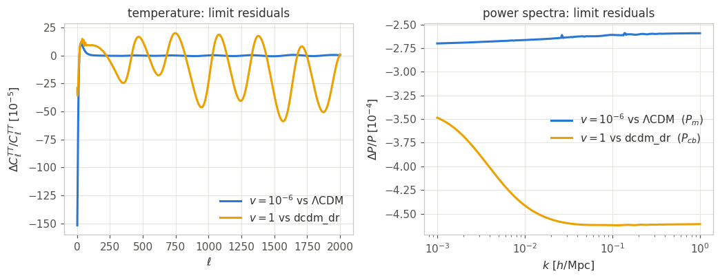
Three limits pin the implementation against known answers (run in full by scripts/validate_dcdm_wdm.py; reproduced here visually):

1. \(v_{\rm kick}\to0\): the daughters are born at rest — indistinguishable from stable CDM with the same total \(\omega_m\).

2. \(v_{\rm kick}=1\) (\(\varepsilon=0\)): massless daughters — the model degenerates to the long-standing dcdm_dr implementation (cold DM → dark radiation).

3. \(f\to0\): no unstable component — ΛCDM.

A convention note for limit 2: the two codes classify the massless daughters differently. dcdm_wdm treats them as (warm) matter — they enter \(P_m\) with their full \(\delta\rho/\rho\), per the standard CLASS convention for ncdm — while dcdm_dr treats them as dark radiation, excluded from \(P_m\). At \(v_{\rm kick}=1\) this bookkeeping difference reaches 18% in \(P_m\) even though the dynamics agree (\(C_\ell^{TT}\) to \(5.5\times10^{-4}\)). The convention-free comparison is \(P_{cb}\) (CDM+baryons), which excludes the daughters in both codes and agrees to \(3.1\times10^{-4}\). (Adding dcdm_wdm also required exposing \(P_{cb}\) for composite-wrapped warm species — the new has_warm_matter() collection property.)

lim0 = run(ddm_pars(f=0.3, inv_gamma_gyr=GYR / 100.0, vkick=1e-6))
lim1 = run(ddm_pars(f=0.3, inv_gamma_gyr=GYR / 100.0, vkick=1.0))
dr = run({"Omega_cdm": OMEGA_DM * 0.7, "Omega_ini_dcdm": OMEGA_DM * 0.3,
          "Gamma_dcdm": 100.0})
print(f"runs: {lim0['t']:.1f} s, {lim1['t']:.1f} s, {dr['t']:.1f} s")

ll = np.arange(2, 2001)
fig, (ax1, ax2) = plt.subplots(1, 2, figsize=(9.6, 3.8))
ax1.plot(ll, 1e5 * (lim0["lensed"]["tt"][2:2001] / lcdm["lensed"]["tt"][2:2001] - 1),
         color=C1, label="$v=10^{-6}$ vs $\\Lambda$CDM")
ax1.plot(ll, 1e5 * (lim1["lensed"]["tt"][2:2001] / dr["lensed"]["tt"][2:2001] - 1),
         color=C3, label="$v=1$ vs dcdm_dr")
ax1.set_xlabel("$\\ell$"); ax1.set_ylabel("$\\Delta C_\\ell^{TT}/C_\\ell^{TT}\\;[10^{-5}]$")
ax1.set_title("temperature: limit residuals")
ax1.legend()

ax2.semilogx(lim0["k"], 1e4 * (lim0["pk"] / lcdm["pk"] - 1), color=C1,
             label="$v=10^{-6}$ vs $\\Lambda$CDM  ($P_m$)")
ax2.semilogx(lim1["k"], 1e4 * (lim1["pk_cb"] / dr["pk_cb"] - 1), color=C3,
             label="$v=1$ vs dcdm_dr  ($P_{cb}$)")
ax2.set_xlabel("$k$ [$h$/Mpc]"); ax2.set_ylabel("$\\Delta P/P\\;[10^{-4}]$")
ax2.set_title("power spectra: limit residuals")
ax2.legend()
fig.tight_layout()
print("max |dTT/TT| v->0:", np.max(np.abs(lim0['lensed']['tt'][2:2001]/lcdm['lensed']['tt'][2:2001]-1)))
print("max |dTT/TT| v=1 vs dr:", np.max(np.abs(lim1['lensed']['tt'][2:2001]/dr['lensed']['tt'][2:2001]-1)))
print("max |dPcb/Pcb| v=1 vs dr:", np.max(np.abs(lim1['pk_cb']/dr['pk_cb']-1)))

runs: 8.5 s, 34.9 s, 1.5 s
max |dTT/TT| v->0: 0.0015171686922818006
max |dTT/TT| v=1 vs dr: 0.0005868944903114626
max |dPcb/Pcb| v=1 vs dr: 0.000462361976924508

4. Recreating the physics panels of arXiv:2606.14849 (Fig. 3)

The paper’s Fig. 3 shows fractional deviations from ΛCDM in \(P(k)\), \(C_\ell^{TT}\) and \(C_L^{\phi\phi}\) for \(f=0.1\) and lifetimes \(\Gamma^{-1} \in \{0.1, 1, 10\}\) Gyr, with \(\varepsilon\) chosen so that \(v_{\rm kick}\) sits at their \(1\sigma\) CMB upper limit. The \(1\sigma\) values are read off their Fig. 2 (left panel, \(f=0.1\) curve) — approximately \(v/c \approx 0.03,\ 0.011,\ 0.02\) for \(\Gamma^{-1} = 0.1,\ 1,\ 10\) Gyr (the bound is tightest near \(\Gamma^{-1}\sim1\) Gyr, where decays complete just as lensing becomes sensitive).

Expected physics (paper §IV.B): suppression of \(P(k)\) onsets near the free-streaming scale \(k_{\rm fs} = 2\pi/\lambda_{\rm fs}\) (their Eq. 1, dashed vertical lines below); the suppression propagates to \(C_L^{\phi\phi}\) at the ~5–10% level over Planck’s lensing range \(L\lesssim400\); the low-\(\ell\) TT changes stay small. Earlier decays (shorter \(\Gamma^{-1}\)) push \(k_{\rm fs}\) to smaller scales and accumulate more growth suppression.

\[\lambda_{\rm fs} = \frac{v_{\rm kick}}{1+z_d}\int_0^{z_d}\frac{1+z}{H(z)}\,\mathrm{d}z, \qquad H(z_d)=\Gamma,\qquad \ell_{\rm fs} \sim \pi\,\chi_*/\lambda_{\rm fs}.\]

models = [(0.1, 0.03, C1), (1.0, 0.011, C2), (10.0, 0.02, C3)]
results = []
for inv_gamma, vk, color in models:
    r = run(ddm_pars(f=0.1, inv_gamma_gyr=inv_gamma, vkick=vk), background=True)
    results.append(r)
    print(f"Gamma^-1 = {inv_gamma:5.1f} Gyr, v = {vk}: {r['t']:.1f} s")


def freestream_scales(r, inv_gamma, vk):
    # z_d (H = Gamma), k_fs in h/Mpc, and l_fs ~ pi chi*/lambda_fs (paper Eq. 1)
    bgd = r["bg"]
    zb = bgcol(bgd, "z")
    Hb = bgcol(bgd, "H [1/Mpc]")
    Gamma_code = (GYR / inv_gamma) * 1e3 / 299792458.0
    z_d = zb[np.argmin(np.abs(Hb - Gamma_code))]
    sel = zb <= z_d
    zz, HH = zb[sel][::-1], Hb[sel][::-1]  # ascending z from 0 to z_d
    lam = vk / (1 + z_d) * np.trapezoid((1 + zz) / HH, zz)  # comoving Mpc
    chi_star = r["derived"]["ra_rec"]  # comoving Mpc
    k_fs = 2 * np.pi / lam / BASE["h"]  # h/Mpc
    return z_d, k_fs, np.pi * chi_star / lam


fig, axes = plt.subplots(3, 1, figsize=(7.2, 9.6), sharex=False)
LL = np.arange(2, 2001)
Lpp = np.arange(2, 1001)
for (inv_gamma, vk, color), r in zip(models, results):
    lab = f"$\\Gamma^{{-1}}={inv_gamma:g}\\,$Gyr, $v={vk}$"
    z_d, k_fs, l_fs = freestream_scales(r, inv_gamma, vk)
    print(f"Gamma^-1={inv_gamma:5.1f} Gyr: z_d={z_d:8.1f}, k_fs={k_fs:.3f} h/Mpc, l_fs={l_fs:.0f}")
    axes[0].semilogx(r["k"], 100 * (r["pk"] / lcdm["pk"] - 1), color=color, label=lab)
    if k_fs < 1.0:
        axes[0].axvline(k_fs, color=color, ls="--", lw=1.0, alpha=0.7)
    axes[1].plot(LL, 100 * (r["lensed"]["tt"][2:2001] / lcdm["lensed"]["tt"][2:2001] - 1),
                 color=color, label=lab)
    axes[2].plot(Lpp, 100 * (r["raw"]["pp"][2:1001] / lcdm["raw"]["pp"][2:1001] - 1),
                 color=color, label=lab)
    if l_fs < 1000:
        axes[2].axvline(l_fs, color=color, ls="--", lw=1.0, alpha=0.7)

axes[0].set_xlabel("$k$ [$h$/Mpc]")
axes[0].set_ylabel("$\\Delta P_m/P_m$ [%]")
axes[0].set_title("matter power (dashed: $k_{\\rm fs}=2\\pi/\\lambda_{\\rm fs}$)")
axes[0].legend(fontsize=8.5)
axes[1].set_xlabel("$\\ell$")
axes[1].set_ylabel("$\\Delta C_\\ell^{TT}/C_\\ell^{TT}$ [%]")
axes[1].set_title("lensed temperature")
axes[2].axvspan(2, 400, color="#f3f2ef", zorder=0)
axes[2].set_xlabel("$L$")
axes[2].set_ylabel("$\\Delta C_L^{\\phi\\phi}/C_L^{\\phi\\phi}$ [%]")
axes[2].set_title("lensing potential (shaded: Planck conservative range $L \\leq 400$; "
                  "dashed: $\\ell_{\\rm fs}$)")
axes[2].set_xlim(2, 1000)
fig.suptitle("arXiv:2606.14849 Fig. 3 physics panels — $f=0.1$, $v_{\\rm kick}$ at the "
             "paper's $1\\sigma$ bounds", y=1.0, fontsize=11)
fig.tight_layout()

Gamma^-1 =   0.1 Gyr, v = 0.03: 11.7 s
Gamma^-1 =   1.0 Gyr, v = 0.011: 11.2 s
Gamma^-1 =  10.0 Gyr, v = 0.02: 11.1 s
Gamma^-1=  0.1 Gyr: z_d=    39.6, k_fs=0.151 h/Mpc, l_fs=711
Gamma^-1=  1.0 Gyr: z_d=     7.8, k_fs=0.255 h/Mpc, l_fs=1201
Gamma^-1= 10.0 Gyr: z_d=     0.7, k_fs=0.240 h/Mpc, l_fs=1131

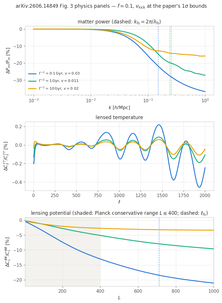
The three panels reproduce the paper’s qualitative anatomy: power suppression switching on around \(k_{\rm fs}\) and saturating at small scales; \(C_L^{\phi\phi}\) suppressed at the several-percent level across Planck’s lensing range (the paper quotes 5–10% for \(1\sigma\) models — the constraining signal); and small low-\(\ell\) TT shifts from the late-time background change. Earlier decays (blue) push the suppression to higher \(k\) and deepen it — the growth-suppression accumulation the paper describes in §IV.B.

5. Momentum-grid convergence and cost

The momentum grid is injection-adapted, not log-spaced in \(q\): bins carry equal decayed fraction \(F = 1-e^{-\Gamma t}\) (a Poisson-process quantile in time), placed at their momenta via a fixed fiducial \(H(t)\) — so the grid is a pure function of \(\Gamma\) alone, invariant of the run’s actual cosmology at fixed \(\Gamma\). q_edge_tol is now the grid-span knob (how far the grid’s realized \(F\)-span may fall short of \([0,1]\) before falling back to a uniform grid); the historical kernel_width parameter is gone — there is no separate kernel-width knob to set.

Energy is injected via a conservative cell-integrated Gaussian (erf) deposit: at a kick \(u_{\rm cut} = \ln(a\,q_{\rm kick})\), the kick’s energy is split across bins by normal-CDF differences at the cell edges, with off-grid tails clamped into the edge bins, so \(\sum_i W_i = 1\) identically (the energy sum rule holds exactly, no renormalization) for every cutoff position. The width is \(\sigma = \mathrm{clamp}(\Delta u_{\rm loc},\,0.03,\,0.25)\) — the analytic local quantile-bin width, floored by the background table’s resolution and capped by the placement-bias budget. On top of that, a static-sparsity floor (\(10^{-12}\) of the deposit, added to every bin before renormalizing) keeps every injection row structurally nonzero: ndf15’s numjac derives the Jacobian’s sparsity pattern from exact zeros and locks it permanently once it repeats, so a moving compact source would lock too narrow a pattern and corrupt the grouped Jacobian once the footprint sweeps on. ∂J/∂\ln q carries the complete two-term derivative — the cell-averaged profile derivative (normal-pdf differences at the edges) and the measure term \(-(3+q^2/\varepsilon^2)J\) coming from \(\mathrm{d}\ln(q^3\varepsilon)/\mathrm{d}\ln q\); an earlier build of this branch omitted the second term, which silently produced a flat \(\sim\!-7.6\%\) low-\(k\) \(P_m\) deficit (now fixed — see the low-\(k\) \(\Lambda\)CDM-anchor numbers quoted below).

Both evolvers integrate this source, since it is smooth (\(C^\infty\)) in time: evolver = 2 (rkdp45) is recommended for routine use (~14\(\times\) faster than the default, cost summary below); the default ndf15 also completes cleanly — its own successful completion is the regression test for a hang that an earlier, non-smooth deposit used to cause at momenta_bins ≳ 48.

Known discrepancy vs the old (master) uniform-grid scheme. Master’s deposit (a \(D\)-renormalized Gaussian, uniform in \(\ln q\)) carries a flat +1.9% \(\langle\beta^2\rangle\) velocity excess relative to its own analytic \(w(z)\) (a momentum-placement bias, the same \(q^3\)-tilt mechanism as above) — invisible to energy conservation (\(\rho_{\rm wdm}\) agrees with the analytic injection integral to \(\lesssim\!10^{-4}\) on both schemes) but it shifts the free-streaming cutoff, so old-vs-new \(P_m(k)\) differ there by construction. The injection-adapted grid here is the validated one: its background \(\rho_{\rm wdm}\) and \(p_{\rm wdm}\) match the analytic monochromatic-kick prediction independently, and its \(P_m(k)\) matches a \(\Lambda\)CDM control at \(k\lesssim0.01\,h\)/Mpc to \(<0.1\%\) (.superpowers/sdd/task-3-diagnosis.md). The standalone convergence harness (dcdm_wdm_convergence.py / _compare.py, re-run on this branch’s fixed build, truth = this grid at 192 bins) puts numbers on it: old-192 vs new-192 max\(|\Delta P_m/P_m|\) is \(1.7\times10^{-3}\) (\(\Gamma^{-1}=0.1\) Gyr, \(v=0.03\)) / \(1.3\times10^{-3}\) (\(\Gamma^{-1}=1\) Gyr, \(v=0.011\)) — and at \(k=0.01\,h\)/Mpc specifically, where the free-streaming cutoff has not yet acted, it is \(\sim\!1.1\times10^{-4}\) for both, confirming the bias is concentrated away from low \(k\) exactly as the mechanism predicts.

Sweeping the momentum-bin count and holding everything else fixed (\(f=0.1\), \(\Gamma^{-1}=1\) Gyr, \(v_{\rm kick}=0.011\) — the same model as the harness’s g1_v0p011), against a 192-bin reference:

BINS_SWEEP = (16, 24, 32, 48, 96)
REF_BINS = 192

conv = {}
for bins in BINS_SWEEP + (REF_BINS,):
    r = run(ddm_pars(f=0.1, inv_gamma_gyr=1.0, vkick=0.011, bins=bins))
    conv[bins] = r
    print(f"bins={bins:4d}: {r['t']:5.1f} s")

# Sequential ramp (single hue, light -> dark): bin count is an ordered/magnitude
# quantity, not a categorical identity, so it gets a sequential encoding rather
# than the notebook's fixed categorical slots (dataviz: "sequential = one hue").
_cmap = matplotlib.colormaps["Blues"]
sweep_colors = [_cmap(0.30 + 0.55 * i / (len(BINS_SWEEP) - 1)) for i in range(len(BINS_SWEEP))]

plt.figure(figsize=(7.0, 4.0))
for bins, color in zip(BINS_SWEEP, sweep_colors):
    plt.semilogx(conv[bins]["k"], 100 * (conv[bins]["pk"] / lcdm["pk"] - 1),
                 color=color, label=f"{bins} bins")
plt.semilogx(conv[REF_BINS]["k"], 100 * (conv[REF_BINS]["pk"] / lcdm["pk"] - 1),
             "--", color=NEUTRAL, lw=1.6, label=f"{REF_BINS} bins (truth)")
plt.xlabel("$k$ [$h$/Mpc]")
plt.ylabel("$\\Delta P_m/P_m$ [%]")
plt.title("momentum-grid convergence ($\\Gamma^{-1}=1$ Gyr, $v=0.011$, $f=0.1$)")
plt.legend(fontsize=8.5)
plt.tight_layout()

print(f"\nself-convergence vs {REF_BINS}-bin reference:")
ref_pk = conv[REF_BINS]["pk"]
for bins in BINS_SWEEP:
    d = np.max(np.abs(conv[bins]["pk"] / ref_pk - 1))
    print(f"  max |P_{bins}/P_{REF_BINS} - 1| = {d:.2e}")

bins=  16:   2.1 s
bins=  24:   2.9 s
bins=  32:   3.6 s
bins=  48:   5.3 s
bins=  96:  11.2 s
bins= 192:  24.5 s

self-convergence vs 192-bin reference:
  max |P_16/P_192 - 1| = 3.16e-03
  max |P_24/P_192 - 1| = 1.99e-03
  max |P_32/P_192 - 1| = 1.38e-03
  max |P_48/P_192 - 1| = 7.90e-04
  max |P_96/P_192 - 1| = 2.62e-04

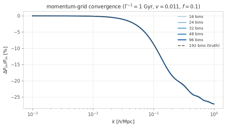
The full accuracy-vs-bins sweep (dcdm_wdm_convergence.py / _compare.py, this branch’s fixed build vs the same 192-bin truth) puts numbers on the curves above. At the 1% target the injection-adapted grid needs 16 bins for both fiducial models (\(\Gamma^{-1}=0.1\) Gyr, \(v=0.03\) and \(\Gamma^{-1}=1\) Gyr, \(v=0.011\), this cell’s own model) versus 70–73 bins for the old uniform-\(\ln q\) grid — a 4.4–4.6\(\times\) reduction. At 0.3%/0.1% the new grid reaches them within the swept range (17–40 bins); the old grid’s error is still above 0.3% even at 96 bins (only dropping to ~0.13–0.17% by 192 bins — the residual discussed above, diluted into a sub-percent \(P_m(k)\) imprint because the unstable fraction is only \(f=0.1\) of the dark matter here).

model	target	old bins	new bins	reduction
\(\Gamma^{-1}=0.1\) Gyr, \(v=0.03\)	1.0%	73	16	4.6\(\times\)
\(\Gamma^{-1}=0.1\) Gyr, \(v=0.03\)	0.3% / 0.1%	not reached by 96 bins	16 / 21	—
\(\Gamma^{-1}=1\) Gyr, \(v=0.011\)	1.0%	70	16	4.4\(\times\)
\(\Gamma^{-1}=1\) Gyr, \(v=0.011\)	0.3% / 0.1%	not reached by 96 bins	17 / 40	—

Cost summary (Apple Silicon, single-threaded per run, l_max_scalars = 2500, lensed spectra + \(P(k)\)):

configuration	wall time
ΛCDM reference	~2 s
dcdm_wdm, 96 bins, evolver = 2 (RK45, recommended)	~4 s
dcdm_wdm, 96 bins, default ndf15	~58 s

ndf15’s implicit machinery (numerical Jacobians + LU on ~1700 equations per mode) is wasted here — the daughter hierarchy is not stiff. evolver = 2 agrees with ndf15 to \(3.5\times10^{-5}\) on all observables.

6. Known limitations and follow-ups

• Synchronous gauge only (input guard rejects Newtonian). The \(\ell=1\) injection source \(\propto\theta_{\rm dcdm}\) is omitted — exact in synchronous gauge where \(\theta_{\rm dcdm}\equiv0\).

• No tensor contribution from the daughters (their anisotropic stress is neglected for tensor modes; they are empty until late times).

• No fluid approximation: MCMC-grade speed would want an Abellán-style viscous-fluid mode for the daughters — a natural follow-up now that the exact reference exists (this notebook’s runs at 4 s each are already MCMC-plausible with evolver = 2).

• Unequal daughter masses (paper footnote 1) are not implemented — the symmetric two-body case of the paper’s main text is.

• The \(P_m\) convention for relativistic daughters (counted as warm matter) differs from dcdm_dr’s dark-radiation classification — §3. For physical kick velocities (\(v\lesssim0.1\)) the daughters are non-relativistic at late times and \(P_m\) is unambiguous.

• Old (master) grid comparison: the uniform-\(\ln q\) grid’s \(\sim\)+1.9% \(\langle\beta^2\rangle\) deposit bias (§5 above) means old-vs-new \(P_m(k)\) differ near the free-streaming cutoff by construction, not by regression — the injection-adapted grid here is the one independently validated against analytic background predictions and a low-\(k\) \(\Lambda\)CDM anchor.

Numerical-robustness notes (relevant to anyone extending the species; details in the commit messages): the daughter’s per-bin distribution values are seeded at \(10^{-10}\) (kFSeed — the stiff evolver’s error weights choke on components starting at exact zero); the injection deposit’s Gaussian pdf/cdf arguments are clamped (exp at argument\(^2/2\ge60\), erf at \(|x|>8\) — extreme arguments are unsafe under -ffast-math); and every injection row carries a \(10^{-12}\) static-sparsity floor so ndf15’s numjac never locks a too-narrow Jacobian sparsity pattern as the deposit’s footprint moves across the grid (§5).

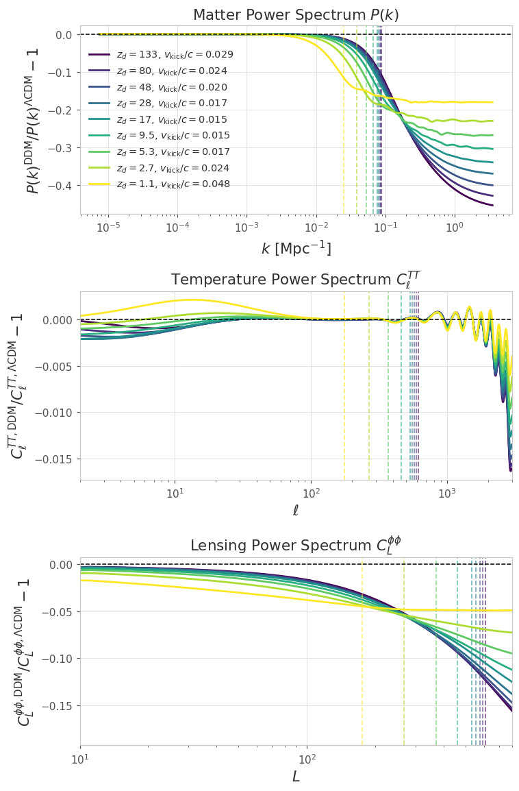
7. The published Fig. 3, model by model

Section 4 recreated the figure’s anatomy from three models guessed off the paper’s Fig. 2; this section runs the exact nine models of the published figure. The legend values \((z_d,\ v_{\rm kick}/c)\) are

\[(133, 0.029),\ (80, 0.024),\ (48, 0.020),\ (28, 0.017),\ (17, 0.015),\]

\[(9.5, 0.015),\ (5.3, 0.017),\ (2.7, 0.024),\ (1.1, 0.048),\]

with \(f=0.1\) and the Planck 2018 best-fit fiducial, including the 0.06 eV neutrino — declared dot-style (nu.type = ncdm_standard, nu.m = 0.06) because the legacy N_ncdm key collides with dot-instance parsing when a ddm.* instance is present. The decay rate follows from the paper’s definition \(\Gamma = H(z_d)\); on this background the nine \(z_d\) values map onto an almost exactly \(10^{1/3}\)-spaced lifetime grid \(\Gamma^{-1} = 0.0164 \to 7.64\) Gyr — strong evidence this is the mapping the authors used.

Two conventions were pinned down by pixel-measuring the published PNG (arXiv-2606.14849v1/DESIDDM/cmb_3panel.png):

• The dashed free-streaming markers use \(\lambda_{\rm fs} = 2\times\) [Eq. (1) integral]. (The paper’s Eq. (1) as printed and its quoted matter-domination limit \(\lambda_{\rm fs}\approx 22{,}000\,(v/c)/\sqrt{1+z_d}\ h^{-1}\)Mpc differ by exactly a factor of 2; the figure follows the latter.) The \(P(k)\) panel marks \(k_{\rm fs}=2\pi/\lambda_{\rm fs}\) and both \(C_\ell\) panels mark \(\ell_{\rm fs}=\pi\chi_*/\lambda_{\rm fs}\); the measured line positions match these to \(\sim\)10%, consistent with the legend’s 2-significant-figure rounding.

• The TT panel is log-\(x\) with \(\ell \in (2, 3000)\); the \(\phi\phi\) panel spans \(L \in (10, 800)\); the \(y\)-ranges are autoscaled.

The figure is produced by the standalone script dcdm_wdm_fig3_9models.py next to this notebook (spectra cached in dcdm_wdm_fig3_cache.npz; delete the cache to force a recompute — about a minute with evolver = 2).

import runpy

# Executes the standalone generator (uses the .npz cache when present; ~1 min otherwise).
fig3 = runpy.run_path("dcdm_wdm_fig3_9models.py", run_name="notebook")

LCDM reference ...
  1.7 s
  z_d =   133, v = 0.029: Gamma^-1 =  0.0164 Gyr, 17.5 s
  z_d =    80, v = 0.024: Gamma^-1 =  0.0351 Gyr, 17.5 s
  z_d =    48, v = 0.020: Gamma^-1 =  0.0749 Gyr, 17.5 s
  z_d =    28, v = 0.017: Gamma^-1 =  0.1649 Gyr, 17.7 s
  z_d =    17, v = 0.015: Gamma^-1 =  0.3377 Gyr, 17.7 s
  z_d =   9.5, v = 0.015: Gamma^-1 =  0.7582 Gyr, 17.8 s
  z_d =   5.3, v = 0.017: Gamma^-1 =  1.6268 Gyr, 18.0 s
  z_d =   2.7, v = 0.024: Gamma^-1 =  3.5558 Gyr, 18.2 s
  z_d =   1.1, v = 0.048: Gamma^-1 =  7.6450 Gyr, 19.2 s
cached spectra in /home/au192734/runners/runner4/_work/CLASSpp/CLASSpp/doc/site/models/dcdm_wdm_fig3_cache.npz
z_d =   133: Gamma^-1 =  0.0164 Gyr, k_fs = 0.0883 1/Mpc, l_fs = 612
z_d =    80: Gamma^-1 =  0.0351 Gyr, k_fs = 0.0854 1/Mpc, l_fs = 592
z_d =    48: Gamma^-1 =  0.0749 Gyr, k_fs = 0.0830 1/Mpc, l_fs = 576
z_d =    28: Gamma^-1 =  0.1649 Gyr, k_fs = 0.0797 1/Mpc, l_fs = 553
z_d =    17: Gamma^-1 =  0.3377 Gyr, k_fs = 0.0767 1/Mpc, l_fs = 532
z_d =   9.5: Gamma^-1 =  0.7582 Gyr, k_fs = 0.0660 1/Mpc, l_fs = 458
z_d =   5.3: Gamma^-1 =  1.6268 Gyr, k_fs = 0.0535 1/Mpc, l_fs = 371
z_d =   2.7: Gamma^-1 =  3.5558 Gyr, k_fs = 0.0385 1/Mpc, l_fs = 267
z_d =   1.1: Gamma^-1 =  7.6450 Gyr, k_fs = 0.0253 1/Mpc, l_fs = 176
wrote /home/au192734/runners/runner4/_work/CLASSpp/CLASSpp/doc/site/models/dcdm_wdm_fig3_9models.png
wrote /home/au192734/runners/runner4/_work/CLASSpp/CLASSpp/doc/site/models/dcdm_wdm_fig3_9models.pdf

Agreement — and one genuine discrepancy

Panel by panel against the published figure:

• \(P(k)\): matches curve-for-curve — plateau depths from \(-0.18\) (\(z_d=1.1\)) to \(-0.46\) (\(z_d=133\)), common crossing at \(k\approx0.15\,\mathrm{Mpc}^{-1}\), onset at the \(k_{\rm fs}\) markers.

• \(C_L^{\phi\phi}\): matches — crossing at \(L\approx250\), earliest decay reaching \(-0.16\).

• \(C_\ell^{TT}\), \(\ell\gtrsim50\): matches, including the lensing-smoothing oscillations growing to \(-1.7\%\) at \(\ell=3000\).

• \(C_\ell^{TT}\), \(\ell\lesssim50\): disagrees for the early decayers. The published panel shows \(+0.8\%/{+1.1\%}\) at \(\ell=2\) for \(z_d=133/80\) — with non-monotonic ordering (80 above 133, 28 above 48) — while we find \(\lesssim10^{-4}\) there. The late decayers agree: our \(z_d=1.1\) model reproduces the published yellow \(+0.2\%\) bump at \(\ell\approx10\)–\(15\).

Four quantitative arguments that the published low-\(\ell\) excess is an artifact of CLASSIER-DDM’s background solution rather than physics missing here:

1. Energy conservation. Two daughters of total mass \(\varepsilon m_\chi\) shed only the kinetic fraction: the asymptotic mass loss is \(f\,(1-\varepsilon)\approx f\,v_{\rm kick}^2/2 \approx 4\times10^{-5}\) of the DM for the most extreme model (\(z_d=133\), \(v=0.029\)). Our background confirms \(\Delta\rho_m/\rho_m = 5\)–\(9\times10^{-5}\) (including mid-decay transients). Calibration runs give a low-\(\ell\) response \(\Delta C_2/C_2 \approx 0.5\,(\Delta\Omega_m/\Omega_m)\) for a deficit established early (constant at late times, as for \(z_d\gtrsim80\)): the published \(+0.8\)–\(1.1\%\) would need \(\Delta\Omega_m/\Omega_m\sim2\%\) — i.e. the sector losing \(\sim\)20% of its energy, \(v_{\rm eff}\sim0.6\) instead of \(0.029\).

2. The paper’s own numbers. §V states the bounds limit the mass loss to \(\Delta\Omega_m/\Omega_m \lesssim 0.1\%\) — itself \(\sim\)20× larger than energy conservation gives at these \((f, v)\), yet still capping the \(\ell=2\) response at \(\sim+0.05\%\), an order of magnitude below their own panel.

3. The known strong-late-ISW benchmark. dcdm_dr at the same \(\Gamma^{-1}=7.6\,\)Gyr, \(f=0.1\) gives \(+9.7\%\) at \(\ell=2\) — the familiar large DCDM\(\to\)DR signal — because there the sector loses its entire rest energy. Two massive daughters suppress exactly this by \((1-\varepsilon)\approx v_{\rm kick}^2/2\), and deficits developing during the \(\Lambda\) era are \(\sim\)30× more ISW-efficient per unit deficit than early-established ones — which is why only the late decayers show a visible (and mutually agreeing) low-\(\ell\) signal.

4. Closure-condition conventions cannot bridge the gap. The paper’s basis fixes \(\omega_\Lambda\) (h derived); a CLASS-style closure fixes \(h\) (\(\Omega_\Lambda\) derived). Explicit runs in both conventions at the true deficit move \(C_2\) by \(+3\times10^{-5}\) and \(-1\times10^{-5}\) respectively. Incidentally, our runs effectively sit in the paper’s convention: the composite’s fixed-point shoot of the \(\Omega_{\rm dcdmwdm}\) closure reserve only engages when its residual exceeds fzero_Newton’s tolF \(=10^{-3}\) (it does for \(v\gtrsim0.3\); verified re-closing exactly at \(v=0.5\) and \(v=1\)). At physical kicks \(\rho_\Lambda\) keeps the Omega_ini seed and the realized \(H_0\) absorbs \(-\delta_{\rm kin}/2\approx-1.4\times10^{-5}\) — cosmologically negligible, but worth knowing. (Related: the \(v=1\) validation floor of \(5.5\times10^{-4}\) in §3 is partly dcdm_dr’s own shooting tolerance — its \(v=1\) run realizes \(H_0\) off by \(-3.6\times10^{-4}\) while the composite converges to \(10^{-9}\).)

Bottom line: the perturbation physics of dcdm_wdm reproduces the published figure quantitatively; the residual low-\(\ell\) TT disagreement for early decays is internally inconsistent within the paper itself and is being raised with the authors.